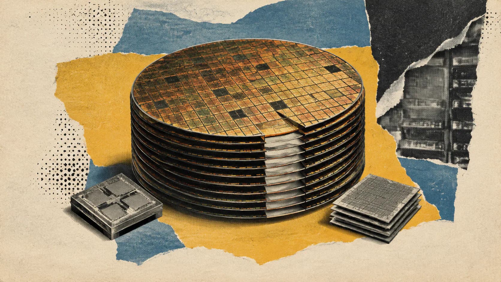
Cerebras published an engineering walkthrough on October 22, 2026, showing how an approximately three-trillion-parameter Kimi K3 model could fit across 59 WSE-3T wafer-scale chips. Each wafer has 44 GB of on-chip SRAM, so the model must span many chips even with its weights compressed to four bits each.
The guide explains the placement decisions behind that number: two linear-attention layers share a wafer, while each dense-attention layer gets a wafer with room reserved for its attention cache. Weights remain resident, and intermediate activations move between pipeline stages.
This is an illustrative deployment guide from Cerebras, not a Kimi model launch. Its most useful contribution is the separation between two engineering problems: fitting the model’s weights and retaining enough request state to serve concurrent users.
Why the Example Needs 59 Wafers
Cerebras bases its worked example on three assumptions:
- 4-bit model weights, reducing the raw storage required for parameters.
- An 8-bit KV cache, specifying the storage precision for cached attention keys and values.
- A 256k-token average request size, used to size request-related memory.
The model has 69 linear-attention layers and 24 dense, full-attention layers, for 93 layers in total. Cerebras divides the raw weight payload evenly across those layers to get an approximate per-layer size.
| Calculation | Result |
|---|---|
| Three trillion parameters × 4 bits ÷ 8 bits per byte | 1.5 trillion bytes |
| Raw weight payload in decimal units | 1,500 GB, or 1.5 TB |
| 1,500 GB ÷ 93 layers | About 16.1 GB per layer |
| 69 linear-attention layers, two per wafer | 35 wafers |
| 24 dense-attention layers, one per wafer | 24 wafers |
| Total | 59 wafers |
The 35-wafer subtotal rounds upward: 34 wafers hold 68 linear-attention layers, leaving one more layer for another wafer.
The approximately 16 GB layer size is the guide’s averaging simplification, not an independently verified inventory of every layer’s storage. Likewise, the 1.5 TB calculation describes raw four-bit parameter data. It is not a complete runtime memory budget.
The important architectural choice appears after that arithmetic. Two roughly 16 GB layers fit inside 44 GB, but Cerebras only pairs the linear-attention layers. Dense layers need substantial additional space for request caches. That choice produces the 59-wafer layout described in the guide.
My view is that this is the number worth examining, ahead of the headline speed claim. It shows how the model’s attention design affects hardware placement, even when the total parameter count stays fixed.
Dense Attention Makes Free Memory a Local Resource
Each dense-attention layer stores keys and values for the tokens in every active request. As a request’s retained context grows, its KV cache grows too.
Linear attention uses a different mechanism. Cerebras describes a small, fixed-size state for each request, avoiding a cache that expands with every additional token. Fixed-size still means some memory per request; it does not mean zero request-related storage.
| Layer type | Illustrative placement | Memory left after approximate weights | Main request-state consideration |
|---|---|---|---|
| Linear attention | Two layers per wafer | About 12 GB | Fixed-size state per request |
| Dense attention | One layer per wafer | About 28 GB | KV cache grows with retained tokens and active requests |
Those headroom figures are simple subtractions from 44 GB. They are nominal space before accounting for other runtime allocations.
Across 59 wafers, the stated SRAM capacity adds up to 2,596 GB, or about 2.6 TB. Comparing that with 1.5 TB of raw weights suggests roughly 1.1 TB remains across the system. But that subtraction hides the placement constraint: spare SRAM is distributed across particular wafers, and the cache belongs with the layer that uses it in this design.
A dense layer cannot automatically use all the spare capacity elsewhere in the pipeline. Each dense-layer wafer must accommodate its own portion of every active request’s cache.
That gives the guide a practical implication: total memory capacity alone is an inadequate serving-capacity metric. The useful question is how much usable cache memory remains at the most constrained dense-attention stage.
Weights Stay Resident While Activations Move
Cerebras separates model placement from request movement. Its compiler maps layers across regions of wafers, and its runtime determines the path that tokens follow between those stages.
Once the model is loaded, the described inference path keeps layer weights resident in on-chip SRAM. A wafer computes its assigned layers and sends the resulting activations, the intermediate numerical representations of the request, to the next wafer.
In the guide’s simplified example:
- The first wafer computes layers 1 and 2.
- It sends the resulting activations to the second wafer.
- The second wafer computes layers 3 and 4.
- Processing continues through the remaining mapped layers until the final stage produces the next token.
Cerebras says those inter-wafer transfers use RDMA over Ethernet, with roughly two microseconds per hop. That is a vendor-reported transfer figure, not a measurement of a full token-generation pass.
The company summarizes the boundary traffic clearly: “Only activations cross from one wafer to the next.” The claim concerns the described model-execution path, where whole layers generally fit locally and their weights do not need to be streamed between wafers during each pass. (Cerebras guide)
Keeping weights local limits what must cross the network. It does not eliminate interconnect latency, local computation or scheduling costs. A two-microsecond hop therefore cannot be used on its own to calculate an end-to-end output rate.
Multiple Requests Keep the Pipeline Occupied
A single token moves through the model’s stages in order. Sending only one request through the entire system before starting another would leave much of the hardware idle.
Cerebras instead describes overlapping work from different requests. At one instant, stage three might process request A, stage two request B, and stage one request C. All three stages can perform useful work simultaneously.
Each stage can also process a micro-batch, a small group of requests. The guide gives a rough scheduling relationship: requests in flight are approximately the number of pipeline stages multiplied by the micro-batch size.
That relationship describes how work can occupy the pipeline. Memory still has to support those requests.
It is also important to keep wafers, layers and stages separate. The guide uses layer-sized stages to explain the idea, then says production deployments use much finer-grained stages and many more of them. The 59-wafer count should not be read as an exact count of production scheduling stages.
Cerebras describes the micro-batching tradeoff as smaller groups favoring individual-request speed and larger groups increasing total throughput. That distinction matters for anyone evaluating AI products: a system can complete more work across many users without making one user’s response proportionally faster.
For ordinary autoregressive generation, a request needs its previous output before producing its next token. Filling the pipeline with other requests improves utilization, while each individual request still pays for its own forward pass.
KV Cache Sets a Separate Concurrency Ceiling
Every active request needs cache space on every dense-attention layer. That requirement persists even while the request is being processed somewhere else in the pipeline.
For example, a request currently executing on a later wafer still needs the earlier dense layers’ stored keys and values for its next token. Moving computation forward does not free all the request’s earlier caches.
Frequently Asked Questions
3 questions
1Does Every Three-Trillion-Parameter Model Need 59 Wafers?
No. This count follows Cerebras’s illustrative Kimi K3 layer mix, quantization and memory placement. Different attention designs, layer sizes or precision choices can change the mapping.